
After an artificial intelligence algorithm is selected and trained, the final step is to test the results. When we started, we split the data into two groups – training data and testing data. Now that we’re done training the algorithm with the training data, we can use the test data for testing. During the testing phase, the algorithm will predict the output and compare to the actual answer. In most datasets, some data will be incorrectly predicted.
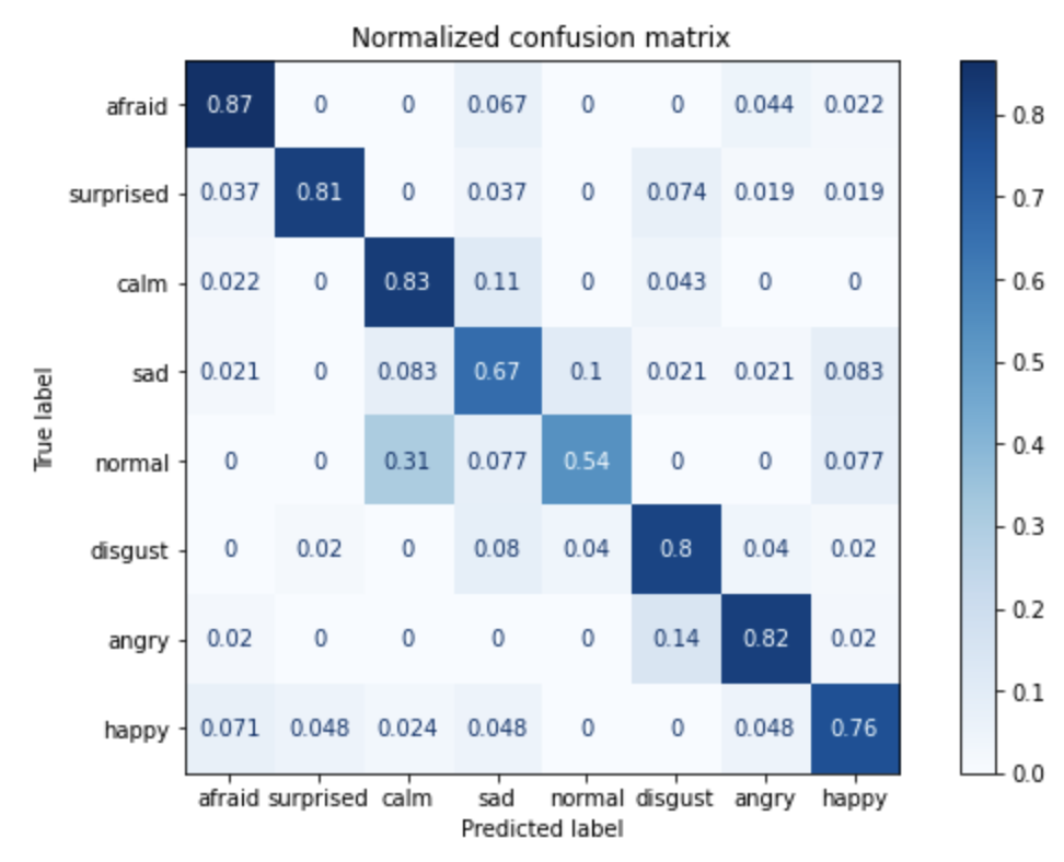
The confusion matrix allows us to get a better understanding of the incorrectly predicted data by showing what was predicted vs the actual value. In the below matrix, I trained a neural network to determine the mood of an individual based on characteristics of their voice. The Y axis shows the actual mood of the speaker and the X axis shows the predicted value. From my matrix, I can see that my model does a reasonable job predicting fear, surprise, calm, angry, and happy but performs more poorly for normal and sad. Since my matrix is normalized, the numbers indicate percentages. For example, 87 percent of afraid speakers were correctly identified.
Creating the above confusion matrix is simple with Scikit-Learn. Start by selecting the best model and then predict the output using that classifier. For my code below, I show both the normalized and standard confusion matrix using the plot_confusion_matrix function.
# PICK BEST PREDICTION MODEL
classifier = mlp

# predict value
pred = classifier.predict(X_test)

# plot non-normalized confusion matrix
titles_options = [("Confusion matrix, without normalization", None),
                  ("Normalized confusion matrix", 'true')]
for title, normalize in titles_options:
    disp = plot_confusion_matrix(classifier, X_test, y_test,
                                 display_labels=data[predictionField].unique(),
                                 cmap=plt.cm.Blues,
                                 normalize=normalize)
    disp.ax_.set_title(title)

plt.show()
With the above matrix, I can now go back to the beginning and make changes as necessary. For this matrix, I may collect more samples for the categories that were incorrectly predicted. Or, I may try different settings for my neural network. This process continues – collecting data, tuning parameters, and testing – until the solution meets the requirements for the project.
Conclusion
If you’ve been following along in this series, you should now have a basic understand of artificial intelligence. Additionally, you should be able to create a neural network for a dataset using Scikit-Learn and Jupyter Notebook. All that remains is to find some data and create your own models. One place to start is data.gov – a US government site with a variety of data sources. Have fun!