What is Computer Vision?

Computer Vision is a rapidly growing technology field that most people know little about. While Computer Vision has been around since the 1960s, it’s growth really exploded with the creation of the OpenCV library. This library provides the tools necessary for software engineers to create Computer Vision applications.

But what is Computer Vision? Computer Vision is a mix of hardware and software tools that are used to identify objects from a photo or camera input. One of the more well-known applications of Computer Vision is in self-driving cars. In a self-driving car, numerous cameras collect video inputs. The video streams are then examined to find objects such as road signs, people, stop lights, lines on the road, and other data that would be essential for safe driving.

However, this technology isn’t just available in self-driving cars. A vehicle I rented a few months ago was able to read speed limit signs as I passed by and display that information on the dash. Additionally, if I failed to signal a lane change, the car would beep when I got close to the line.

Another common place to find Computer Vision is in factory automation. In this setting, specialized programs may monitor products for defects, check the status of machinery for leaks or other problematic conditions, or monitor the actions of people to ensure safe machine operation. With these tools, companies can make better products more safely.

Computer Vision and Artificial Intelligence are also becoming more popular for medical applications. Images of MRI or X-Ray scans can be processed using Computer Vision and AI tools to identify cancerous tumors or other problematic health issues.

From a less practical view, Computer Vision tools are also used to modify videos of user content. This may include things such as adding a hat or making a funny face. Or, it may be used to identify faces in an image for tagging.

Ultimately, Computer Vision technologies are being found in more and more places each day and, when coupled with AI, will ultimately result in a far more technologically advanced world.

Dangers of Artificial Intelligence

Risk/Reward

With the growth of artificial intelligence, one of the subjects we don’t discuss enough is the possible dangers that it may create. While AI may help us better drive our cars or provide a rapid, more accurate diagnosis of medical issues; it may also create problems for society. What are those problems and what should we do to minimize those risks?

Poorly Tested Code

As a software engineer, my biggest worry is that poor-quality code will be widely deployed in artificial intelligence systems. Look around today, and you will see what I mean. I use a Mac, and the current version of Safari is riddled with bugs. Indeed, nearly every application on my computer has several updates per year to address bugs.

This is caused, in part, by the demands of businesses. I have worked for many companies over the years who desired to push out a new version even when some known bugs existed. For the business, this is necessary to ensure they beat the competition to release new features. However, this acceptance of buggy software can be disastrous in the world of AI.

For example, what happens when the artificial intelligence system misdiagnoses cancer? For the individual, this could have life-altering effects. What about the self-driving car? Someone could be hit and killed.

How good is good enough for artificial intelligence? I don’t have an answer, but it is something businesses need to strongly consider as they dive deeper into the world of AI.

Deep Fakes

A growing concern for artificial intelligence is how it could be used by organizations or political entities to persuade consumers or voters. For example, a political adversary of the president could create a fake video of the president engaged in some behavior that would bring discredit upon him. How would the electorate know it is a fake? Even worse, how could our nation’s enemies use fake videos for propaganda purposes here or abroad?

Employment

In many ways, advances in artificial intelligence are very similar to the changes during the industrial revolution. As AI becomes more advanced, we can expect to see more and more jobs performed by intelligent robots or computer systems. While this will benefit businesses who can cut payroll, it will have a negative impact laborers who can easily be replaced.

What Should We Do?

This is just a very small list of potential issues. Indeed, numerous techies have discussed countless other risks we face as we adopt more AI-based systems. But what should we do? The value of AI to our lives will be profound, but we must start to consider how we will address these challenges from both a legal and a societal perspective.

For example, we may need to create laws regarding liability for AI systems to ensure that businesses provide adequate testing before deploying systems. But problems like deep fakes and employment aren’t as easy to fix. We can certainly provide training to individuals who are displaced by AI, but as more and more jobs are replaced, where will all the workers go?

I don’t have the answers. However, I think it is time for techies and non-techies alike to start asking the questions so that we can reap the benefits of improving artificial intelligence while mitigating the potential risks

Basics of Artificial Intelligence – IX

After an artificial intelligence algorithm is selected and trained, the final step is to test the results. When we started, we split the data into two groups – training data and testing data. Now that we’re done training the algorithm with the training data, we can use the test data for testing. During the testing phase, the algorithm will predict the output and compare to the actual answer. In most datasets, some data will be incorrectly predicted.

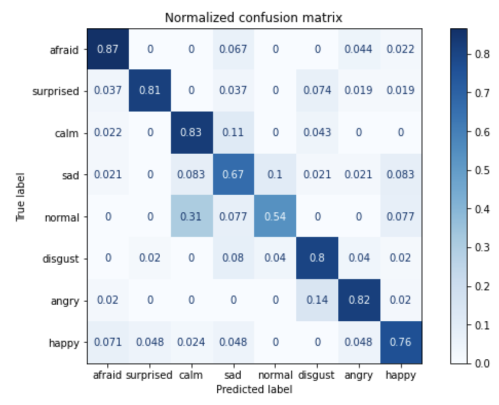
The confusion matrix allows us to get a better understanding of the incorrectly predicted data by showing what was predicted vs the actual value. In the below matrix, I trained a neural network to determine the mood of an individual based on characteristics of their voice. The Y axis shows the actual mood of the speaker and the X axis shows the predicted value. From my matrix, I can see that my model does a reasonable job predicting fear, surprise, calm, angry, and happy but performs more poorly for normal and sad. Since my matrix is normalized, the numbers indicate percentages. For example, 87 percent of afraid speakers were correctly identified.

Creating the above confusion matrix is simple with Scikit-Learn. Start by selecting the best model and then predict the output using that classifier. For my code below, I show both the normalized and standard confusion matrix using the plot_confusion_matrix function.

# PICK BEST PREDICTION MODEL
classifier = mlp

# predict value
pred = classifier.predict(X_test)

# plot non-normalized confusion matrix
titles_options = [("Confusion matrix, without normalization", None),
                  ("Normalized confusion matrix", 'true')]
for title, normalize in titles_options:
    disp = plot_confusion_matrix(classifier, X_test, y_test,
                                 display_labels=data[predictionField].unique(),
                                 cmap=plt.cm.Blues,
                                 normalize=normalize)
    disp.ax_.set_title(title)

plt.show()

With the above matrix, I can now go back to the beginning and make changes as necessary. For this matrix, I may collect more samples for the categories that were incorrectly predicted. Or, I may try different settings for my neural network. This process continues – collecting data, tuning parameters, and testing – until the solution meets the requirements for the project.

Conclusion

If you’ve been following along in this series, you should now have a basic understand of artificial intelligence. Additionally, you should be able to create a neural network for a dataset using Scikit-Learn and Jupyter Notebook. All that remains is to find some data and create your own models. One place to start is data.gov – a US government site with a variety of data sources. Have fun!

Basics of Artificial Intelligence – VIII

Neural Networks are an incredibly useful method for teaching computers how to recognize complex relationships in data. However, in order to get them working properly, you need to know a little more about how they work and how to tune them. This week, we’ll be looking at the two key settings for Neural Networks in scikit-learn.

What Is a Neural Network?

But before we go into those settings, it’s useful to understand what a neural network is. Neural networks are an attempt at modeling computer intelligence on how the human brain works. In our brains, neurons receive electrical impulses from other neurons and, optionally, transmit impulses to other neurons. From there, the process continues with those neurons again deciding how to act on the signal from the previous neuron. Our brains have an estimated 100 billion neurons, all connected to the network to receive and process data.

In the computer, this same idea is replicated with the Neural Network. The inputs values for the network form the first layer of neurons in the artificial brain. From there, one or more hidden layers are created connecting the inputs from the previous stage. Finally, one or more output neurons provide the user with the answer from the digital brain. Of course, this assumes the network has been trained to identify the data.

So, for the developer, the first step to creating the neural network is to determine the number of layers for the network and the number of neurons in each layer. Next, the developer will select from a group of ‘activation functions’ that will define when the neuron fires. The available options are the logistic sigmoid function (logistic), the hyperbolic tan function (tahn) and the rectified linear unit function (relu). Various other parameters can also be set to further tune the network.

Back to the Code

# Create a Neural Network (AKA Multilayer Perceptron or MLP)
# In this example, we will create 3 hidden layers
# The first layer has 512 neurons, the second 128 and the third 16
# Use the rectified linear unit function for activation (RELU)
# For training, iterate no more than 5000000 times
mlp = MLPClassifier( 
    hidden_layer_sizes=(512,128,16)
    activation='relu',
    max_iter=5000000
)

You can see in the above code that we are going to try with 3 layers in the network. This is simply a guess, and we will want to repeatedly attempt different network configurations until we come upon a model that performs to the required specifications.

# Train the neural network
mlp.fit(X_train,y_train)

# Get metrics 
train_metric = mlp.score(X_train, y_train)
test_metric = mlp.score(X_test, y_test)

pred = mlp.predict(X_test)
recall_metric = recall_score(y_test, pred)
precision_metric = precision_score(y_test, pred)

With the above code, we can retrieve scores indicating how well the model did. With a perfect network, all values would be 1 – meaning they were 100% accurate. However, this is rarely the case with actual data. So, you will need to determine what level of accuracy is required. For some networks, 80% may be the limit.

Armed with this information, you should now be able to repeatedly train your network until you have the desired output. With a large dataset, and a large number of configurations, that may take a substantial amount of time. In fact, the training and testing part of AI development is by far the most time consuming.

What’s Next?

Next week, we will look at the final part of developing an AI solution – the Confusion Matrix. This chart will give us a better understanding of how our network is performing than the simple metrics we calculated above.

Basics of Artificial Intelligence – VII

Last week, we used Python libraries to import the data, set the input and out values for the computer to learn, and split the data into groups. Next, we will actually train the computer to learn the relationships. For this, we can use a variety of different tools. While each one has its pros and cons, the novice can simply run each one and determine which one provides the best results. In addition, we will print the results for analysis.

Logistic Regression

# train the model
logreg = LogisticRegression()
logreg.fit(X_train, y_train)

# print accuracy
train_metric = logreg.score(X_train, y_train)
test_metric = logreg.score(X_test, y_test)
print('Accuracy of Logistic regression classifier on training set: {:.2f}'.format(train_metric))
print('Accuracy of Logistic regression classifier on test set: {:.2f}'.format(test_metric))

# print recall
pred = logreg.predict(X_test)
recall_metric = recall_score(y_test, pred, average=recall_average)
precision_metric = precision_score(y_test, pred, average=recall_average)
print('Recall of Logistic regression classifier on test set: {:.2f}'.format(recall_metric))
print('Precision of Logistic regression classifier on test set: {:.2f}'.format(precision_metric))

Decision Tree Classifier

# train the model
clf = DecisionTreeClassifier().fit(X_train, y_train)

# print overall accuracy
train_metric = clf.score(X_train, y_train)
test_metric = clf.score(X_test, y_test)
print('Accuracy of Decision Tree classifier on training set: {:.2f}'.format(test_metric))
print('Accuracy of Decision Tree classifier on test set: {:.2f}'.format(train_metric))

# print recall/precision
pred = clf.predict(X_test)
recall_metric = recall_score(y_test, pred, average=recall_average)
precision_metric = precision_score(y_test, pred, average=recall_average)
print('Recall of Decision Tree classifier on test set: {:.2f}'.format(recall_metric))
print('Precision of Decision Tree classifier on test set: {:.2f}'.format(precision_metric))

Linear Discriminant Analysis

# train the model
lda = LinearDiscriminantAnalysis()
lda.fit(X_train, y_train)

# print overall accuracy
train_metric = lda.score(X_train, y_train)
test_metric = lda.score(X_test, y_test)
print('Accuracy of LDA classifier on training set: {:.2f}'.format(train_metric))
print('Accuracy of LDA classifier on test set: {:.2f}'.format(test_metric))

# print recal
pred = lda.predict(X_test)
recall_metric = recall_score(y_test, pred, average=recall_average)
precision_metric = precision_score(y_test, pred, average=recall_average)
print('Recall of LDA classifier on test set: {:.2f}'.format(recall_metric))
print('Precision of LDA classifier on test set: {:.2f}'.format(precision_metric))

Neural Network

# activation - ‘identity’, ‘logistic’, ‘tanh’, ‘relu’

mlp = MLPClassifier( 
    hidden_layer_sizes=(512,768,1024,512,128,16)
    activation='relu',
    learning_rate='adaptive',
    max_iter=5000000
)

mlp.fit(X_train,y_train)

# print overall accuracy
train_metric = mlp.score(X_train, y_train)
test_metric = mlp.score(X_test, y_test)
print('Accuracy of Neural Network classifier on training set: {:.2f}'.format(train_metric))
print('Accuracy of Neural Network classifier on test set: {:.2f}'.format(test_metric))

# print recall
pred = mlp.predict(X_test)
recall_metric = recall_score(y_test, pred, average=recall_average)
precision_metric = precision_score(y_test, pred, average=recall_average)
print('Recall of Neural Network classifier on test set: {:.2f}'.format(recall_metric))
print('Precision of Neural Network classifier on test set: {:.2f}'.format(precision_metric))

What We did

You will notice that much of the code above is very similar. This is part of what makes Scikit-Learn such an amazing framework – it’s relatively easy to change between Artificial Intelligence algorithms. In addition to the above algorithms, you can also use Support Vector Machines, Naive Bayes, K-Nearest Neighbor, and many more.

Once you’ve run the training, the scores show how each algorithm performed after it was trained. On any given data set, a different algorithm may work better. This is another benefit to Scikit-Learn – the easy access to a variety of models allows for experimentation to find the best model.

What Next?

While much of underlying math for these algorithms is well outside the scope of knowledge for most, it is useful to understand how Neural Networks operate. They are one of the more interesting implements of AI, and can be tuned to work with lots of data. However, that tuning requires some knowledge of what a Neural Network is and how it works. That’s what we’ll look at next week.

Basics of Artificial Intelligence – VI

Last week, we looked at languages used for artificial intelligence development. While there are numerous options available, Python has some of the best tools and is the easiest for the beginner to get started with quickly. However, setup can be quite a bit of work. First, setup Python and a development environment – I strongly recommend Jupyter, but VS Code is ok too. Next, begin installing all the necessary libraries – numpy, pandas, and sklearn. You may also wish to install matplotlib and seaborn. When you’ve got all the libraries installed, you can create a block of code in Jupyter to include all the necessary imports in your project such as what I have below. Some of these libraries are large, so you can prune the list to include only the tools you need.

Of particular interest are the sklearn modules. In this section, you will see imports for a variety of different AI algorithms including logistic regression, decision trees, nearest neighbors, linear discriminant analysis, naïve Bayes, and neural networks. These libraries will do the bulk of the work for us with little effort.

Import Libraries

import numpy as np
import matplotlib.pyplot as plt
import matplotlib as mpl
from matplotlib import cm
import seaborn as sns
import pandas as pd
import patsy

import itertools as it
import collections as co
import functools as ft
import os.path as osp

import glob
import textwrap

from sklearn.model_selection import train_test_split, cross_val_score
from sklearn.neural_network import MLPClassifier
from sklearn.mixture import GaussianMixture
from sklearn.preprocessing import MinMaxScaler, StandardScaler
from sklearn.ensemble import VotingClassifier, AdaBoostClassifier
from sklearn.linear_model import LogisticRegression
from sklearn.tree import DecisionTreeClassifier
from sklearn.neighbors import KNeighborsClassifier
from sklearn.discriminant_analysis import LinearDiscriminantAnalysis
from sklearn.naive_bayes import GaussianNB
from sklearn.pipeline import make_pipeline
from sklearn.ensemble import BaggingClassifier
from sklearn.svm import SVC
from sklearn.metrics import classification_report
from sklearn.metrics import precision_score, recall_score
from sklearn.metrics import f1_score, accuracy_score
from sklearn.metrics import confusion_matrix
from sklearn.metrics import plot_confusion_matrix

Load Data

The next step for any AI project is to import the data and manipulate as needed

# import the data file from CSV format
data = pd.read_csv(open("data.csv", "rb"))

# show the number of records
recordCount = len(data.index)
print("Record Count: {:d}".format(recordCount))

# optional removal of data 
# this will remove all records with a FIELD_VALUE for FIELD_NAME
# data = data.drop(data[data.FIELD_NAME == 'FIELD_VALUE'].index)

# add optional flags for processing
# add a boolean field of true where COLUMN_NAME = VALUE
data.insert(loc=0, column='COLUMN_NAME', value=(data.mood == 'VALUE'))

# show the new record count
newCount = len(data.index)
print("Filtered Count: {:d}".format(recordCount - newCount))

Set Prediction Field & Input Fields

Now that you have loaded the data and manipulated as necessary, it’s time to setup the information for prediction. That will consist of two parts – the field to predict and the values to use for the prediction. So, if I want to determine the value of a house, the prediction value would be the cost and the input fields would include square footage, yard size, number of rooms, etc. In the code snippet below, I will set the fields for predicting home price.

# CSV field to predict
predictionField = 'home_value'

# CSV fields to use for prediction
feature_names = ['square_footage', 'yard_size', 'num_room', 'num_bath']

# extract data into feature set and prediction value (X,y)
X = data[feature_names]
y = data[predictionField]

Split Into Groups

The next important step is to split the data into two groups – training data and test data. The training data will be used by the AI algorithm to ‘learn’ the data. Then, the test data is used to see how well the algorithm actually did in learning the data relationships.

# split into groups
X_train, X_test, y_train, y_test = train_test_split(X, y)

# scale data
scaler = MinMaxScaler()
X_train = scaler.fit_transform(X_train)
X_test = scaler.transform(X_test)

Next Steps

So far, we have loaded the necessary libraries, loaded the data, updated the data to exclude any records we don’t ant, added fields as necessary to augment the data, separated the data into features and prediction fields, and broke the data into groups for training. The next step is where the magic happens – the artificial intelligence algorithm. We’ll look at that next week…

Basics of Artificial Intelligence – V

Up to this point, we have talked about some of the fundamental algorithms for artificial intelligence and how they can be implemented in Java. Java is a great language for speed and wide usage in the software world. However, Java is not the only choice for implementing artificial intelligence. In this post, we will examine three of the most popular languages for creating artificial intelligence solutions.

Java

Java is one of the most widely used computer programming languages available today. Since it’s development in the 90’s, Java has been widely used for web development as well as for creating cross-platform applications. Java runs in a virtual machine – the Java Virtual Machine (JVM). Any computer that has an implementation of the JVM can run a Java program. Additional languages have been developed that are comparable with the JVM as well including Scala, Groovy, and Kotlin. Java is object oriented, compiled, and strongly typed. Compiled languages are fast, but strongly typed languages can be problematic in artificial intelligence as data structures must be well defined or generics implemented which can complicate code.

R

R is a statistical programming language used more by statisticians than computer programmers. It is designed to deal with matrices of data, and as such is very well suited for AI development. Additionally, R has a multitude of packages that can easily create graphs and charts to help analyze data dependencies. However, where R is lacking is in ease of use. Additionally, R isn’t as well suited for deploying AI applications – but rather for research.

Python

Python has been around since the early 90’s. However, it’s mainstream use has only exploded during the last decade or so. Because of it’s simple syntax, Python has been widely embraced by people outside of the programming community – and in educational settings. Because of this, Python use has exploded for utilities, system administration tasks, automation, REST-based web services, and artificial intelligence. Furthermore, Python has excellent frameworks and tools for AI development. Of particular interest are Jupyter and SciKit Learn. These tools greatly simplify AI development, and allow developers to work on solving problems more quickly than Java and with substantially less setup and expertise.

MATLAB

While talking about AI languages, I must also mention MATLAB or, it’s open source alternative Octave. These platforms are incredibly popular in academic communities. However, MATLAB – and the associated toolkits – are expensive and far more difficult to use than Python. Additionally – like R – they don’t really create deployable solutions for customers. However, if you are a mathematician, you may find MATLAB more to your liking.

Conclusion

When I work on artificial intelligence code, I will often use R and Python. While I have been a Java developer for years, and have implemented various AI solutions using Java, I find it far more complicated than the alternatives. I often use R for analyzing correlation, creating charts, and performing statistical analysis of data using R Studio. Then, when it’s time to actually create the neural network, I will use Python and Jupyter.

If you prefer, AI frameworks are available – or can be created – for any other language. If you want the fastest solution, you may look into C libraries. If you want something that will run on a browser in a website, JavaScript may provide a better solution. In short, there are a variety of options for AI. However, for the novice, you’ll probably not find anything better than Python to get you started.

Basics of Artificial Intelligence – IV

Previously, we examined various functions that are used across a variety of artificial intelligence applications. Today, we’re looking at a specific algorithm. While not typically considered artificial intelligence, linear regression is the most basic means of allowing a computer to learn how to solve a problem. For linear regression, the user provides an array of input values as well as an array of expected output values. In algebra, these would be the x and y values of the equation respectively. Additionally, the user will need to provide a degree for the polynomial. This is the highest exponent for the x value in the equation. For example, a third degree polynomial would be ax^3 + bc^2 + cx + d.

Our first class will be the generic base class shared across all linear regression implementations. In this class, we define a method to calculate the score of a set of values as well as an abstract method to calculate the coefficients. NOTE: Referenced code is available for download from BitBucket.

import com.talixa.techlib.ai.general.Errors;
import com.talixa.techlib.math.Polynomial;

public abstract class PolyFinder {
  protected float[] input;
  protected float[] idealOutput;
  protected float[] actualOutput;
  protected float[] bestCoefficients;
  protected int degree;
	
  public PolyFinder(float[] input, float[] idealOutput, int degree) {
    this.input = input;
    this.idealOutput = idealOutput;
    this.actualOutput = new float[idealOutput.length];
    this.bestCoefficients = new float[degree+1];
    this.degree = degree;
  }

  public abstract float[] getCoefficients(int maxIterations);
	
  protected float calculateScore(float[] coefficients) {
    // iterate through all input values and calculate the output
    // based on the generated polynomials
    for(int i = 0; i < input.length; ++i) {
      actualOutput[i] = Polynomial.calculate(input[i], coefficients);
    }

    // return the error of this set of coefficients
    return Errors.sumOfSquares(idealOutput, actualOutput);
  }
}

Our next step is to create an actual implementation of code to get the coefficients. Multiple method are available, but we will look at the simplest – greedy random training. In greedy random training, the system will generate random values and keep the values with the lowest error score. It’s a trivial implementation and works well for low-order polynomials.

import java.util.Arrays;
import com.talixa.techlib.ai.prng.RandomLCG;

public class PolyGreedy extends PolyFinder {
  private float minX;
  private float maxX;
	
  public PolyGreedy(float[] trainingInput, float[] idealOutput, int degree, float minX, float maxX) {
    super(trainingInput, idealOutput, degree);
    this.minX = minX;
    this.maxX = maxX;
  }
	
  public float[] getCoefficients(int maxIterations) {
    // iterate through the coefficient generator maxIterations times
    for(int i = 0; i < maxIterations; ++i) {
      iterate();
    }
    // return a copy of the best coefficients found
    return Arrays.copyOf(bestCoefficients, bestCoefficients.length);
  }
	
  private void iterate() {
    // get score with current values
    float oldScore = calculateScore(bestCoefficients);
		
    // randomly determine new values
    float[] newCoefficients = new float[degree+1];
    for(int i = 0; i < (degree+1); ++i) {
      newCoefficients[i] = RandomLCG.getNextInt() % (maxX - minX) + minX;
    }
		
    // test score with new values
    float newScore = calculateScore(newCoefficients);
		
    // determine if better match
    if (newScore < oldScore) {
      bestCoefficients = newCoefficients;
    }
  }
}

With the greedy random training, we define the min and max values for the parameters and then iterate over and over selecting random values for the equation. Each time a new value is created, it is compared with the current best score. If this score is better, it becomes the new winner. This algorithm can be run thousands of times to quickly create a set of coefficients to solve the equation.

For many datasets, this can create a workable answer within a short time. However, linear regression works best less complicated datasets were some relationship between the x and y values is known to exist. In cases of multiple input values where the relationship between variables is less clear, other algorithms may provide a better answer.

Basics of Artificial Intelligence – III

Some artificial intelligence algorithms like input values to be normalized. This means that all data is presented within a predefined range, typically either 0 to 1 or -1 to 1. Normalization algorithms take an array of input values and return an array of normalized values.

Denormalization is the opposite process. In denormalization, an input array of normalized values is presented and the original values are returned. Denormalization is useful when the output value of an AI algorithm is normalized. Since the normalized value is not in an expected range, the user must denormalize to determine the real number.

A simple example of number normalization is the Celsius temperature scale. All temperatures where water exists as a liquid exist between the values of 0 and 100. To normalize the temperature for an AI algorithm, I could simply divide each input by 100 to create an array of numbers between 0 and 1. When the output value is .17, the user would denormalize by multiplying by 100 to get a value of 17 degrees.

Of course, most normalization is not this simple, so we use algorithms to do the work.

public static float[] normalizeData(final float[] inputVector, final float minVal, final float maxVal) {
	float[] normalizedData = new float[inputVector.length];
	float dataRange = maxVal - minVal;
	for(int i = 0; i < inputVector.length; ++i) {
		float d = inputVector[i] - minVal;
		float percent = d / dataRange;
		float dnorm = NORMALIZE_RANGE * percent;
		float norm = NORMALIZE_LOW_VALUE + dnorm;
		normalizedData[i] = norm;
	}
	return normalizedData;
}

Note that two constants are defined outside this function. The NORMALIZE_RANGE which is 2 when normalizing to the range of -1 to 1 and the NORMALIZE_RANGE is 1 if we are normalizing to a range of 0 to 1. Additionally, the NORMALIZE_LOW_VALUE is the low value for normalization, either -1 or 0.

In the above normalization function, the user provides an array of input values as well as a min and max value for normalization. Then, we create a new array to hold the normalized values. The code then iterates through each input value and creates the normalized value to add to the normalized data array to return to the user. The actual normalization takes the following steps:

  • subtract the minimum value from the input value
  • divide the output by the data range to determine a percentage
  • multiple the normalized range by the percent
  • Add the value to the normalized low value.

For a concrete example, consider normalizing degrees Fahrenheit. If we were to input an array of daily temperates, we might have [70, 75, 68]. For the normalization range, we would pick 32 and 212. Following the above steps for the first temperature:

  • 70 – 32 = 38
  • 38 / (212 – 32) = .21
  • 2 * .21 = .42
  • -1 + .42 = -.58

If we followed through with the other temperatures, we would end with an output array of [-.58, -.52, -.60]. To denormalize, the below denormalization function can be used. Note, you must use the same min and max values that you used in normalization or your denormalized output value will not be the same scale as your input values!

public static float[] denormalizeData(final float[] normalizedData, final float minVal, final float maxVal) {
	float[] denormalizedData = new float[normalizedData.length];
	float dataRange = maxVal - minVal;
	for(int i = 0; i < normalizedData.length; ++i) {
		float dist = normalizedData[i] - NORMALIZE_LOW_VALUE;
		float pct = dist / NORMALIZE_RANGE;
		float dnorm = pct * dataRange;
		denormalizedData[i] = dnorm + minVal;
	}
	return denormalizedData;
}

This is the most basic normalization function. Other options may be to use the reciprocal of a number (but this only works for number greater than 1 or less than -1) or to use a Z-score.

Basics of Artificial Intelligence – II

Last week, we talked about distance calculations for Artificial Intelligence. Once you’ve learned how to calculate distance, you need to learn how to calculate an overall error for your algorithm. There are three main algorithms for error calculation. Sum of Squares, Mean Squared, and Root Mean Squared. They are all relatively simple, but are key to any Machine Learning algorithm. As an AI algorithm iterates over data time and time again, it will try to find a better solution than the previous iteration. A lower error score indicates a better answer and progress toward the best solution.

The error algorithms are similar to the distance algorithms. However, distance measures how far apart two points are whereas error measures how far the AI output answers are from the expected answers. The three algorithms below show how each error is calculated. Note that each one builds on the one before it. The sum of squares error is – as the name suggests – a summation of the square of the errors of each answer. Note that as the number of answers increases, the sum of squares value will too. Thus, to compare errors with different numbers of values, we need to divide by the number of items to get the mean squared error. Finally, if you want to have a number in a similar range to the original answer, you need to take the square root of the mean squared error.

public static float sumOfSquares(final float[] expected, final float[] actual) {
	float sum = 0;
	for(int i = 0; i < expected.length; ++i) {
		sum += Math.pow(expected[i] - actual[i], 2);
	}
	return sum;
}
	
public static float meanSquared(final float[] expected, final float[] actual) {
	return sumOfSquares(expected, actual)/expected.length;
}
	

public static float rootMeanSquared(final float[] expected, final float[] actual) {
	return (float)Math.sqrt(meanSquared(expected,actual));
}