Category: Programming

Last week, we talked about distance calculations for Artificial Intelligence. Once you’ve learned how to calculate distance, you need to learn how to calculate an overall error for your algorithm. There are three main algorithms for error calculation. Sum of Squares, Mean Squared, and Root Mean Squared. They are all relatively simple, but are key to any Machine Learning algorithm. As an AI algorithm iterates over data time and time again, it will try to find a better solution than the previous iteration. A lower error score indicates a better answer and progress toward the best solution.

The error algorithms are similar to the distance algorithms. However, distance measures how far apart two points are whereas error measures how far the AI output answers are from the expected answers. The three algorithms below show how each error is calculated. Note that each one builds on the one before it. The sum of squares error is – as the name suggests – a summation of the square of the errors of each answer. Note that as the number of answers increases, the sum of squares value will too. Thus, to compare errors with different numbers of values, we need to divide by the number of items to get the mean squared error. Finally, if you want to have a number in a similar range to the original answer, you need to take the square root of the mean squared error.

public static float sumOfSquares(final float[] expected, final float[] actual) {
	float sum = 0;
	for(int i = 0; i < expected.length; ++i) {
		sum += Math.pow(expected[i] - actual[i], 2);
	}
	return sum;
}
	
public static float meanSquared(final float[] expected, final float[] actual) {
	return sumOfSquares(expected, actual)/expected.length;
}
	

public static float rootMeanSquared(final float[] expected, final float[] actual) {
	return (float)Math.sqrt(meanSquared(expected,actual));
}

For the next several weeks, I’m going to write about some basics of artificial intelligence. AI has been around for decades, but has become particularly popular during the last 20 years thanks to advances in computing. In short, artificial intelligence aims to use computers to solve complex problems quicker and more accurately than human can. Early AI was far different than what we have today. Typically, early AI systems would use complex logic programmed into the system to solve problems. Examples include Dijkstra’s Algorithm or the logic programmed into most games. Modern systems, however, are capable of actually learning for themselves given enough data.

Distance Algorithms

The first set of algorithms necessary to understand AI are distance algorithms. These algorithms are used to determine how close a system is to the right answer. This is necessary when an AI system is learning so that it knows how far off the answer it is. The three main distance algorithms are Euclidian, Manhattan, and Chebyshev. Euclidian distance measures distance as a straight line “as the crow flies” between points on a grid. Manhattan distance travels along one axis and then another, like a taxi traversing New York City. Finally, Chebyshev distance travels like a King on a chessboard alternating between each axis as it gets closer to the target.

In each of the code snippets below, written in Java, two vectors are passed in – v1 and v2 – where each vector represents a data point. In each instance, the size of the vector would determine the dimensionality of the data. For example, a float[2] would be a 2-D vector which could be plotted on a cartesian plot.

Euclidian Distance Algorithm

public static float euclidean(final float[] v1, final float[] v2) {
	float sum = 0;
	for(int i = 0; i < v1.length; ++i) {
		sum += (v1[i] - v2[i]) * (v1[i] - v2[i]);
	}
	return (float)Math.sqrt(sum);
}

In the above code, we iterate through two arrays of floating point numbers and then sum the squares of the differences. Finally, return the square root to determine the distance.

Manhattan Distance Algorithm

public static float manhattan(final float[] v1, final float[] v2) {
	float sum = 0;
	for(int i = 0; i < v1.length; ++i) {
		sum += (float)Math.abs(v1[i] - v2[i]);
	}
	return sum;
}

For the Manhattan distance, we calculate and return the sum of the absolute values of the differences.

Chebyshev Distance Algorithm

public static float chebyshev(final float[] v1, final float[] v2) {
	float result = 0;
	for(int i = 0; i < v1.length; ++i) {
		float d = Math.abs(v1[i] - v2[i]);
		result = Math.max(d, result);
	}
	return result;
}

Finally, in the Chebyshev algorithm, the value is the maximum dimension in any direction.

Many people are interested in artificial intelligence and machine learning, but what framework should you start out with to hit the ground running fast? Jupyter and Scikit-Learn!

Jupyter

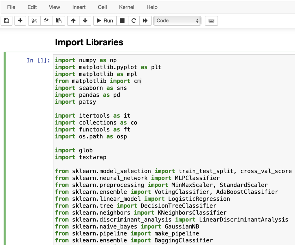
Jupyter is a web-based development environment well-suited for Python development and artificial intelligence. What makes it great for AI development is the nature of the web platform. You can add code blocks, generate images and charts, or add markdown to document what you’re doing. What is also useful is that each block of code within the IDE can be executed as needed by clicking the run button at the top. This is something you will do over and over as you tune your AI parameters to get better accuracy.

The Jupiter Notebook is installed directly on your computer, so you can access local files. This is critical for being able to access the data you will use to train your AI model and ensures optimal performance when using large data sets.

Scikit-Learn

There are countless frameworks for AI, but Scikit-Learn is my favorite. Since it’s a Python-based framework, it’s relatively easy for anyone to work with. Furthermore, since Python is heavily used in artificial intelligence research, you’re using a tool well known to other practitioners in the field. Scikit-Learn supports just about anything you could want for AI including logistic regression, k-nearest neighbors, neural networks, naive bayes, and support vector machines. Even better, Scikit-learn makes it so simple to implement that you don’t really need to know much about the underlying technology.

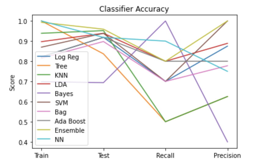
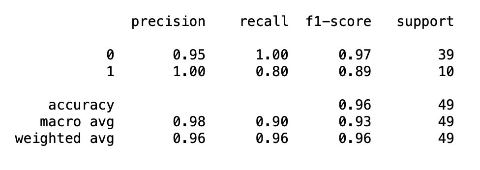
Part of what makes scikit-learn so useful is how easy it is to create charts or graphs. This can include a typical confusion matrix or any plot for your data. This can be really powerful in AI to better understand the data and what relationships may exist.

Getting Started

If you’re interested in getting started, visit jupyter.org to download their IDE. Then, visit scikit-learn.org for installation instructions. If you’re familiar with Python, you’re ready to start with the scikit-learn tutorial on their website. If not, take a trip to YouTube and find some videos on Python development!