Basics of Artificial Intelligence – VI

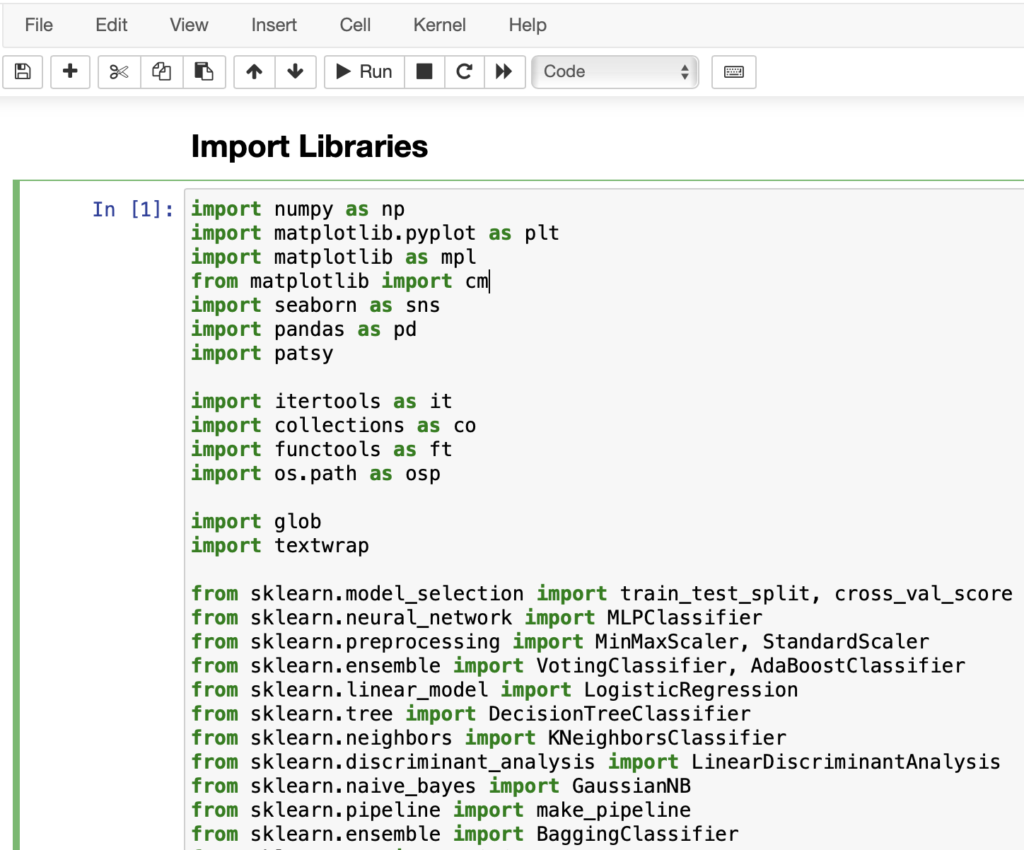
Last week, we looked at languages used for artificial intelligence development. While there are numerous options available, Python has some of the best tools and is the easiest for the beginner to get started with quickly. However, setup can be quite a bit of work. First, setup Python and a development environment – I strongly recommend Jupyter, but VS Code is ok too. Next, begin installing all the necessary libraries – numpy, pandas, and sklearn. You may also wish to install matplotlib and seaborn. When you’ve got all the libraries installed, you can create a block of code in Jupyter to include all the necessary imports in your project such as what I have below. Some of these libraries are large, so you can prune the list to include only the tools you need.

Of particular interest are the sklearn modules. In this section, you will see imports for a variety of different AI algorithms including logistic regression, decision trees, nearest neighbors, linear discriminant analysis, naïve Bayes, and neural networks. These libraries will do the bulk of the work for us with little effort.

Import Libraries

import numpy as np
import matplotlib.pyplot as plt
import matplotlib as mpl
from matplotlib import cm
import seaborn as sns
import pandas as pd
import patsy

import itertools as it
import collections as co
import functools as ft
import os.path as osp

import glob
import textwrap

from sklearn.model_selection import train_test_split, cross_val_score
from sklearn.neural_network import MLPClassifier
from sklearn.mixture import GaussianMixture
from sklearn.preprocessing import MinMaxScaler, StandardScaler
from sklearn.ensemble import VotingClassifier, AdaBoostClassifier
from sklearn.linear_model import LogisticRegression
from sklearn.tree import DecisionTreeClassifier
from sklearn.neighbors import KNeighborsClassifier
from sklearn.discriminant_analysis import LinearDiscriminantAnalysis
from sklearn.naive_bayes import GaussianNB
from sklearn.pipeline import make_pipeline
from sklearn.ensemble import BaggingClassifier
from sklearn.svm import SVC
from sklearn.metrics import classification_report
from sklearn.metrics import precision_score, recall_score
from sklearn.metrics import f1_score, accuracy_score
from sklearn.metrics import confusion_matrix
from sklearn.metrics import plot_confusion_matrix

Load Data

The next step for any AI project is to import the data and manipulate as needed

# import the data file from CSV format
data = pd.read_csv(open("data.csv", "rb"))

# show the number of records
recordCount = len(data.index)
print("Record Count: {:d}".format(recordCount))

# optional removal of data 
# this will remove all records with a FIELD_VALUE for FIELD_NAME
# data = data.drop(data[data.FIELD_NAME == 'FIELD_VALUE'].index)

# add optional flags for processing
# add a boolean field of true where COLUMN_NAME = VALUE
data.insert(loc=0, column='COLUMN_NAME', value=(data.mood == 'VALUE'))

# show the new record count
newCount = len(data.index)
print("Filtered Count: {:d}".format(recordCount - newCount))

Set Prediction Field & Input Fields

Now that you have loaded the data and manipulated as necessary, it’s time to setup the information for prediction. That will consist of two parts – the field to predict and the values to use for the prediction. So, if I want to determine the value of a house, the prediction value would be the cost and the input fields would include square footage, yard size, number of rooms, etc. In the code snippet below, I will set the fields for predicting home price.

# CSV field to predict
predictionField = 'home_value'

# CSV fields to use for prediction
feature_names = ['square_footage', 'yard_size', 'num_room', 'num_bath']

# extract data into feature set and prediction value (X,y)
X = data[feature_names]
y = data[predictionField]

Split Into Groups

The next important step is to split the data into two groups – training data and test data. The training data will be used by the AI algorithm to ‘learn’ the data. Then, the test data is used to see how well the algorithm actually did in learning the data relationships.

# split into groups
X_train, X_test, y_train, y_test = train_test_split(X, y)

# scale data
scaler = MinMaxScaler()
X_train = scaler.fit_transform(X_train)
X_test = scaler.transform(X_test)

Next Steps

So far, we have loaded the necessary libraries, loaded the data, updated the data to exclude any records we don’t ant, added fields as necessary to augment the data, separated the data into features and prediction fields, and broke the data into groups for training. The next step is where the magic happens – the artificial intelligence algorithm. We’ll look at that next week…

Basics of Artificial Intelligence – V

Up to this point, we have talked about some of the fundamental algorithms for artificial intelligence and how they can be implemented in Java. Java is a great language for speed and wide usage in the software world. However, Java is not the only choice for implementing artificial intelligence. In this post, we will examine three of the most popular languages for creating artificial intelligence solutions.

Java

Java is one of the most widely used computer programming languages available today. Since it’s development in the 90’s, Java has been widely used for web development as well as for creating cross-platform applications. Java runs in a virtual machine – the Java Virtual Machine (JVM). Any computer that has an implementation of the JVM can run a Java program. Additional languages have been developed that are comparable with the JVM as well including Scala, Groovy, and Kotlin. Java is object oriented, compiled, and strongly typed. Compiled languages are fast, but strongly typed languages can be problematic in artificial intelligence as data structures must be well defined or generics implemented which can complicate code.

R

R is a statistical programming language used more by statisticians than computer programmers. It is designed to deal with matrices of data, and as such is very well suited for AI development. Additionally, R has a multitude of packages that can easily create graphs and charts to help analyze data dependencies. However, where R is lacking is in ease of use. Additionally, R isn’t as well suited for deploying AI applications – but rather for research.

Python

Python has been around since the early 90’s. However, it’s mainstream use has only exploded during the last decade or so. Because of it’s simple syntax, Python has been widely embraced by people outside of the programming community – and in educational settings. Because of this, Python use has exploded for utilities, system administration tasks, automation, REST-based web services, and artificial intelligence. Furthermore, Python has excellent frameworks and tools for AI development. Of particular interest are Jupyter and SciKit Learn. These tools greatly simplify AI development, and allow developers to work on solving problems more quickly than Java and with substantially less setup and expertise.

MATLAB

While talking about AI languages, I must also mention MATLAB or, it’s open source alternative Octave. These platforms are incredibly popular in academic communities. However, MATLAB – and the associated toolkits – are expensive and far more difficult to use than Python. Additionally – like R – they don’t really create deployable solutions for customers. However, if you are a mathematician, you may find MATLAB more to your liking.

Conclusion

When I work on artificial intelligence code, I will often use R and Python. While I have been a Java developer for years, and have implemented various AI solutions using Java, I find it far more complicated than the alternatives. I often use R for analyzing correlation, creating charts, and performing statistical analysis of data using R Studio. Then, when it’s time to actually create the neural network, I will use Python and Jupyter.

If you prefer, AI frameworks are available – or can be created – for any other language. If you want the fastest solution, you may look into C libraries. If you want something that will run on a browser in a website, JavaScript may provide a better solution. In short, there are a variety of options for AI. However, for the novice, you’ll probably not find anything better than Python to get you started.

Basics of Artificial Intelligence – IV

Previously, we examined various functions that are used across a variety of artificial intelligence applications. Today, we’re looking at a specific algorithm. While not typically considered artificial intelligence, linear regression is the most basic means of allowing a computer to learn how to solve a problem. For linear regression, the user provides an array of input values as well as an array of expected output values. In algebra, these would be the x and y values of the equation respectively. Additionally, the user will need to provide a degree for the polynomial. This is the highest exponent for the x value in the equation. For example, a third degree polynomial would be ax^3 + bc^2 + cx + d.

Our first class will be the generic base class shared across all linear regression implementations. In this class, we define a method to calculate the score of a set of values as well as an abstract method to calculate the coefficients. NOTE: Referenced code is available for download from BitBucket.

import com.talixa.techlib.ai.general.Errors;
import com.talixa.techlib.math.Polynomial;

public abstract class PolyFinder {
  protected float[] input;
  protected float[] idealOutput;
  protected float[] actualOutput;
  protected float[] bestCoefficients;
  protected int degree;
	
  public PolyFinder(float[] input, float[] idealOutput, int degree) {
    this.input = input;
    this.idealOutput = idealOutput;
    this.actualOutput = new float[idealOutput.length];
    this.bestCoefficients = new float[degree+1];
    this.degree = degree;
  }

  public abstract float[] getCoefficients(int maxIterations);
	
  protected float calculateScore(float[] coefficients) {
    // iterate through all input values and calculate the output
    // based on the generated polynomials
    for(int i = 0; i < input.length; ++i) {
      actualOutput[i] = Polynomial.calculate(input[i], coefficients);
    }

    // return the error of this set of coefficients
    return Errors.sumOfSquares(idealOutput, actualOutput);
  }
}

Our next step is to create an actual implementation of code to get the coefficients. Multiple method are available, but we will look at the simplest – greedy random training. In greedy random training, the system will generate random values and keep the values with the lowest error score. It’s a trivial implementation and works well for low-order polynomials.

import java.util.Arrays;
import com.talixa.techlib.ai.prng.RandomLCG;

public class PolyGreedy extends PolyFinder {
  private float minX;
  private float maxX;
	
  public PolyGreedy(float[] trainingInput, float[] idealOutput, int degree, float minX, float maxX) {
    super(trainingInput, idealOutput, degree);
    this.minX = minX;
    this.maxX = maxX;
  }
	
  public float[] getCoefficients(int maxIterations) {
    // iterate through the coefficient generator maxIterations times
    for(int i = 0; i < maxIterations; ++i) {
      iterate();
    }
    // return a copy of the best coefficients found
    return Arrays.copyOf(bestCoefficients, bestCoefficients.length);
  }
	
  private void iterate() {
    // get score with current values
    float oldScore = calculateScore(bestCoefficients);
		
    // randomly determine new values
    float[] newCoefficients = new float[degree+1];
    for(int i = 0; i < (degree+1); ++i) {
      newCoefficients[i] = RandomLCG.getNextInt() % (maxX - minX) + minX;
    }
		
    // test score with new values
    float newScore = calculateScore(newCoefficients);
		
    // determine if better match
    if (newScore < oldScore) {
      bestCoefficients = newCoefficients;
    }
  }
}

With the greedy random training, we define the min and max values for the parameters and then iterate over and over selecting random values for the equation. Each time a new value is created, it is compared with the current best score. If this score is better, it becomes the new winner. This algorithm can be run thousands of times to quickly create a set of coefficients to solve the equation.

For many datasets, this can create a workable answer within a short time. However, linear regression works best less complicated datasets were some relationship between the x and y values is known to exist. In cases of multiple input values where the relationship between variables is less clear, other algorithms may provide a better answer.

Basics of Artificial Intelligence – III

Some artificial intelligence algorithms like input values to be normalized. This means that all data is presented within a predefined range, typically either 0 to 1 or -1 to 1. Normalization algorithms take an array of input values and return an array of normalized values.

Denormalization is the opposite process. In denormalization, an input array of normalized values is presented and the original values are returned. Denormalization is useful when the output value of an AI algorithm is normalized. Since the normalized value is not in an expected range, the user must denormalize to determine the real number.

A simple example of number normalization is the Celsius temperature scale. All temperatures where water exists as a liquid exist between the values of 0 and 100. To normalize the temperature for an AI algorithm, I could simply divide each input by 100 to create an array of numbers between 0 and 1. When the output value is .17, the user would denormalize by multiplying by 100 to get a value of 17 degrees.

Of course, most normalization is not this simple, so we use algorithms to do the work.

public static float[] normalizeData(final float[] inputVector, final float minVal, final float maxVal) {
	float[] normalizedData = new float[inputVector.length];
	float dataRange = maxVal - minVal;
	for(int i = 0; i < inputVector.length; ++i) {
		float d = inputVector[i] - minVal;
		float percent = d / dataRange;
		float dnorm = NORMALIZE_RANGE * percent;
		float norm = NORMALIZE_LOW_VALUE + dnorm;
		normalizedData[i] = norm;
	}
	return normalizedData;
}

Note that two constants are defined outside this function. The NORMALIZE_RANGE which is 2 when normalizing to the range of -1 to 1 and the NORMALIZE_RANGE is 1 if we are normalizing to a range of 0 to 1. Additionally, the NORMALIZE_LOW_VALUE is the low value for normalization, either -1 or 0.

In the above normalization function, the user provides an array of input values as well as a min and max value for normalization. Then, we create a new array to hold the normalized values. The code then iterates through each input value and creates the normalized value to add to the normalized data array to return to the user. The actual normalization takes the following steps:

  • subtract the minimum value from the input value
  • divide the output by the data range to determine a percentage
  • multiple the normalized range by the percent
  • Add the value to the normalized low value.

For a concrete example, consider normalizing degrees Fahrenheit. If we were to input an array of daily temperates, we might have [70, 75, 68]. For the normalization range, we would pick 32 and 212. Following the above steps for the first temperature:

  • 70 – 32 = 38
  • 38 / (212 – 32) = .21
  • 2 * .21 = .42
  • -1 + .42 = -.58

If we followed through with the other temperatures, we would end with an output array of [-.58, -.52, -.60]. To denormalize, the below denormalization function can be used. Note, you must use the same min and max values that you used in normalization or your denormalized output value will not be the same scale as your input values!

public static float[] denormalizeData(final float[] normalizedData, final float minVal, final float maxVal) {
	float[] denormalizedData = new float[normalizedData.length];
	float dataRange = maxVal - minVal;
	for(int i = 0; i < normalizedData.length; ++i) {
		float dist = normalizedData[i] - NORMALIZE_LOW_VALUE;
		float pct = dist / NORMALIZE_RANGE;
		float dnorm = pct * dataRange;
		denormalizedData[i] = dnorm + minVal;
	}
	return denormalizedData;
}

This is the most basic normalization function. Other options may be to use the reciprocal of a number (but this only works for number greater than 1 or less than -1) or to use a Z-score.

Basics of Artificial Intelligence – II

Last week, we talked about distance calculations for Artificial Intelligence. Once you’ve learned how to calculate distance, you need to learn how to calculate an overall error for your algorithm. There are three main algorithms for error calculation. Sum of Squares, Mean Squared, and Root Mean Squared. They are all relatively simple, but are key to any Machine Learning algorithm. As an AI algorithm iterates over data time and time again, it will try to find a better solution than the previous iteration. A lower error score indicates a better answer and progress toward the best solution.

The error algorithms are similar to the distance algorithms. However, distance measures how far apart two points are whereas error measures how far the AI output answers are from the expected answers. The three algorithms below show how each error is calculated. Note that each one builds on the one before it. The sum of squares error is – as the name suggests – a summation of the square of the errors of each answer. Note that as the number of answers increases, the sum of squares value will too. Thus, to compare errors with different numbers of values, we need to divide by the number of items to get the mean squared error. Finally, if you want to have a number in a similar range to the original answer, you need to take the square root of the mean squared error.

public static float sumOfSquares(final float[] expected, final float[] actual) {
	float sum = 0;
	for(int i = 0; i < expected.length; ++i) {
		sum += Math.pow(expected[i] - actual[i], 2);
	}
	return sum;
}
	
public static float meanSquared(final float[] expected, final float[] actual) {
	return sumOfSquares(expected, actual)/expected.length;
}
	

public static float rootMeanSquared(final float[] expected, final float[] actual) {
	return (float)Math.sqrt(meanSquared(expected,actual));
}

Basics of Artificial Intelligence – I

For the next several weeks, I’m going to write about some basics of artificial intelligence. AI has been around for decades, but has become particularly popular during the last 20 years thanks to advances in computing. In short, artificial intelligence aims to use computers to solve complex problems quicker and more accurately than human can. Early AI was far different than what we have today. Typically, early AI systems would use complex logic programmed into the system to solve problems. Examples include Dijkstra’s Algorithm or the logic programmed into most games. Modern systems, however, are capable of actually learning for themselves given enough data.

Distance Algorithms

The first set of algorithms necessary to understand AI are distance algorithms. These algorithms are used to determine how close a system is to the right answer. This is necessary when an AI system is learning so that it knows how far off the answer it is. The three main distance algorithms are Euclidian, Manhattan, and Chebyshev. Euclidian distance measures distance as a straight line “as the crow flies” between points on a grid. Manhattan distance travels along one axis and then another, like a taxi traversing New York City. Finally, Chebyshev distance travels like a King on a chessboard alternating between each axis as it gets closer to the target.

In each of the code snippets below, written in Java, two vectors are passed in – v1 and v2 – where each vector represents a data point. In each instance, the size of the vector would determine the dimensionality of the data. For example, a float[2] would be a 2-D vector which could be plotted on a cartesian plot.

Euclidian Distance Algorithm

public static float euclidean(final float[] v1, final float[] v2) {
	float sum = 0;
	for(int i = 0; i < v1.length; ++i) {
		sum += (v1[i] - v2[i]) * (v1[i] - v2[i]);
	}
	return (float)Math.sqrt(sum);
}

In the above code, we iterate through two arrays of floating point numbers and then sum the squares of the differences. Finally, return the square root to determine the distance.

Manhattan Distance Algorithm

public static float manhattan(final float[] v1, final float[] v2) {
	float sum = 0;
	for(int i = 0; i < v1.length; ++i) {
		sum += (float)Math.abs(v1[i] - v2[i]);
	}
	return sum;
}

For the Manhattan distance, we calculate and return the sum of the absolute values of the differences.

Chebyshev Distance Algorithm

public static float chebyshev(final float[] v1, final float[] v2) {
	float result = 0;
	for(int i = 0; i < v1.length; ++i) {
		float d = Math.abs(v1[i] - v2[i]);
		result = Math.max(d, result);
	}
	return result;
}

Finally, in the Chebyshev algorithm, the value is the maximum dimension in any direction.

Jupyter & Scikit-Learn for Artificial Intelligence

Jupiter

Many people are interested in artificial intelligence and machine learning, but what framework should you start out with to hit the ground running fast? Jupyter and Scikit-Learn!

Jupyter

Jupyter is a web-based development environment well-suited for Python development and artificial intelligence. What makes it great for AI development is the nature of the web platform. You can add code blocks, generate images and charts, or add markdown to document what you’re doing. What is also useful is that each block of code within the IDE can be executed as needed by clicking the run button at the top. This is something you will do over and over as you tune your AI parameters to get better accuracy.

The Jupiter Notebook is installed directly on your computer, so you can access local files. This is critical for being able to access the data you will use to train your AI model and ensures optimal performance when using large data sets.

Scikit-Learn

There are countless frameworks for AI, but Scikit-Learn is my favorite. Since it’s a Python-based framework, it’s relatively easy for anyone to work with. Furthermore, since Python is heavily used in artificial intelligence research, you’re using a tool well known to other practitioners in the field. Scikit-Learn supports just about anything you could want for AI including logistic regression, k-nearest neighbors, neural networks, naive bayes, and support vector machines. Even better, Scikit-learn makes it so simple to implement that you don’t really need to know much about the underlying technology.

Part of what makes scikit-learn so useful is how easy it is to create charts or graphs. This can include a typical confusion matrix or any plot for your data. This can be really powerful in AI to better understand the data and what relationships may exist.

Getting Started

If you’re interested in getting started, visit jupyter.org to download their IDE. Then, visit scikit-learn.org for installation instructions. If you’re familiar with Python, you’re ready to start with the scikit-learn tutorial on their website. If not, take a trip to YouTube and find some videos on Python development!

Skills All Developers Should Know

Tools

When I talk with developers, it’s amazing how many of them are disappointed with the limited job opportunities available to them. Often, the problem is that they lack many of the common skills required to be an effective programmer in today’s market. These developers have managed to become specialists in a very specific technology stack which isn’t widely used elsewhere. I’ll tell them some things they should learn, and – surprisingly – they’ll often argue that the specific skill I mentioned isn’t that useful. What are those skills?

HTML

First and foremost, every developer today needs to know HTML. In our web-based world, it’s hard to find work that doesn’t require HTML at some point. This is obviously true for web development, but is equally valuable with hybrid mobile technologies such as Cordova or Ionic. Or, maybe you need to create documentation for you application that will be accessed on the web.

JavaScript

While every developer may use a different programming language for backend development, we all use JavaScript for web programming. But JavaScript goes well beyond that. Today, JavaScript can be used for developing backend services with Node or even interfacing with Arduino hardware with the Johnny5 library.

Git

Developers need to be comfortable with Git from the command line. GUIs are nice, but when you need to automate a build script or download code from a command prompt on a remote computer, the Git command line is essential.

BASH

Like it or not, much of the cloud runs on Linux servers. As such, a knowledge of BASH is essential in today’s world. While many developers prefer a Windows only world, it’s just not the case when you have to deal with Google or AWS cloud services.

SQL

It’s amazing to me how many junior developers are unfamiliar with SQL. In today’s marketplace, nearly every application needs to interact with a database somewhere. Whether it’s an enterprise application using Oracle or an Android app using SQLite, SQL is the common way to interact with a database.

Conclusion

It may be noted that – other than JavaScript – no programming languages are on the list. Whether you develop in C, C++, Java, Swift or some other language, the above skills will apply. There are countless toolkits and frameworks, languages and environments. However, nearly all of them will require some mix of knowledge of HTML, JavaScript, Git, Bash, and SQL

Simple Text Search

Search

I often need to search a directory of code for instances of a specific word. I like tools that I can use from the command line so that I can execute them from an SSH session across the network. Here’s how I do it.

#!/bin/bash

SAVEIFS=$IFS
IFS=$(echo -en "\n\b")

if [ $# -ne 1 ]
then
        echo Call is: `basename $0` string
else
        for file in `find . -type f | cut -c3-`
        do
                count=`cat "$file" | grep -i $1 | wc -l`
                if [ $count -gt 0 ]
                then
                        echo "******"$file"******"
                        cat "$file" | grep -i $1
                fi
        done
fi
IFS=$SAVEIFS

Line Counting

Codes

A common metric used in software development is lines of code. While it’s not always a useful metric, it’s sometimes nice to know just how large a project is. I have a script I use to count lines of code in a folder. It will iterate through a variety of common file extensions and count all lines of code excluding blank lines. It’s written using sh, so it works on Unix, Linux, or MacOS, and should work on Windows if you have the Bash subsystem installed.

#!/bin/bash

# add additional extensions here
extensions=(bas c cc cob cpp cs cshtml fth f90 go h html java js jsp m pas php pl py sc sh sql ts xhtml)

for extension in ${extensions[@]}
do
  lines=`find . -name "*.$extension" -type f -exec cat {} \; | tr -d '[:blank:]' 2> /dev/null | grep -v '^$' | wc -l `
  if [ $lines -ne 0 ]
  then 
    echo $extension: $lines
  fi
done